











Summary
Databricks Lakebase is managed PostgreSQL inside Databricks that serves Gold-layer lakehouse data to applications with low latency, and synced tables handle the reverse ETL. This guide covers the architecture, a Customer 360 walkthrough, sync mode choice, limits and Lakebase pricing.
Which Lakebase does this guide describes
Everything below describes Lakebase Autoscaling, the current version, and is accurate as of October 2026. Databricks made Lakebase generally available on 22 January 2026. Since 12 March 2026 new instances are created as Autoscaling projects, and existing Provisioned instances were upgraded automatically, with the upgrade completed in July 2026.
Sizing changed with the move. In Lakebase Provisioned, one capacity unit allocated roughly 16 GB of RAM. In Autoscaling, one Compute Unit (CU) allocates roughly 2 GB, so sizing an Autoscaling database with Provisioned numbers puts you off by a factor of eight. Confirm current pricing, region availability and compute sizing in the Databricks documentation before you commit a budget.
The problem: lakehouse analytics your application can’t reach
Modern data platforms handle data engineering, analytics, machine learning and AI well. The last mile is harder: handing a single row to an application in a few milliseconds while a user waits on a page load.
Suppose a Databricks Gold table holds a Customer 360 dataset with customer details, segmentation, churn probability and next-best product. A web application only needs to run:
| SELECT customer_name, customer_segment, churn_probability, recommended_product FROM customer_360 WHERE customer_id = 1001; |
That query is an operational point lookup: one row, one key, one user waiting. A warehouse endpoint is the wrong engine for it. You pay analytical startup cost to fetch a single row, and application developers end up writing retry logic around a system that was never designed to sit in a request path. Latency in that path shows up on the bill too, as one Inferenz team found when it cut DynamoDB costs and improved latency with ElastiCache in an IoT event pipeline.
Databricks Lakebase closes that gap.
What is Databricks Lakebase?
Databricks Lakebase is a fully managed PostgreSQL database integrated with the Databricks Data Intelligence Platform. It keeps analytical work in the Lakehouse and serves the results through PostgreSQL, an open source database that has been ACID compliant since 2001. Lakebase runs PostgreSQL 16, 17 and 18 with more than 50 extensions, including pgvector for vector search and PostGIS for geospatial data.
| Layer | What it handles |
| Lakehouse | Ingestion, large-scale transformation, analytics, machine learning and AI |
| Lakebase | Low-latency lookups, transactions, application state and operational serving |
The split follows the OLTP and OLAP divide. OLTP systems handle short reads and writes on individual records in milliseconds. OLAP systems scan large datasets in seconds to minutes. The Lakehouse takes the second job and Lakebase takes the first.
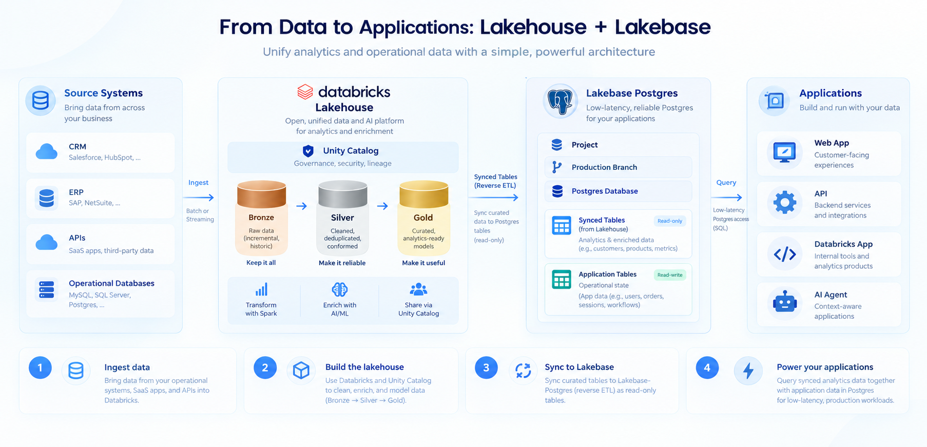
How the Lakehouse and Lakebase connect: from Medallion architecture to serving
Data from CRM platforms, ERP systems, APIs, files and operational databases lands in the Lakehouse and moves through the Medallion architecture. Bronze holds raw ingested data. Silver cleans, standardizes and validates it. Gold holds business-ready datasets: Customer 360, recommendations, risk scores and model predictions.
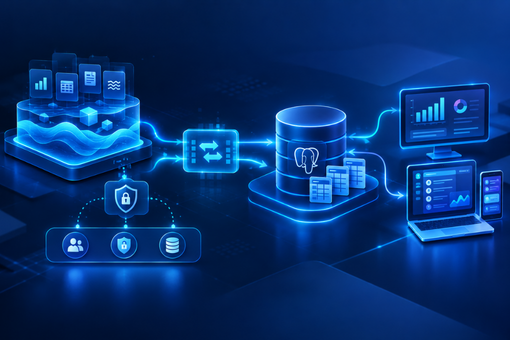
Selected Gold datasets are then synchronized into Lakebase using synced tables, and applications query the resulting PostgreSQL tables over ordinary PostgreSQL connectivity. That detail does more work than it looks like. Application developers keep the drivers, ORMs and connection pools they already know, and never learn a new data access pattern to consume a model output.
The overall pattern, built on a well-run data lake architecture that we had shared a couple of years back now is changed to:
Source Systems → Bronze → Silver → Gold → Synced Tables → Lakebase PostgreSQL → Applications
Inside Lakebase: projects, branches and separated compute
Lakebase Autoscaling uses a project-and-branch architecture with compute separated from storage. A project is the PostgreSQL environment for an application. Within a project, branches serve production, development, testing or feature work.
Branches are copy-on-write, so a development branch is charged storage only for the data that diverges from its parent. That changes team behavior: you stop maintaining a fleet of near-identical PostgreSQL environments and start branching a database the way you branch a repository.
Separating compute from storage makes the rest possible: autoscaling, scale-to-zero, branching, read replicas, high availability, backup and point-in-time restore. It also drives the cost model, covered in the pricing section below.
Lakebase synced tables: reverse ETL from Unity Catalog to PostgreSQL
Say the Lakehouse holds main.gold.customer_360. A custom PySpark or ETL job could export that dataset into an external PostgreSQL instance. A synced table does the same work as a managed object: Databricks handles the synchronization between the Unity Catalog source and its PostgreSQL representation.
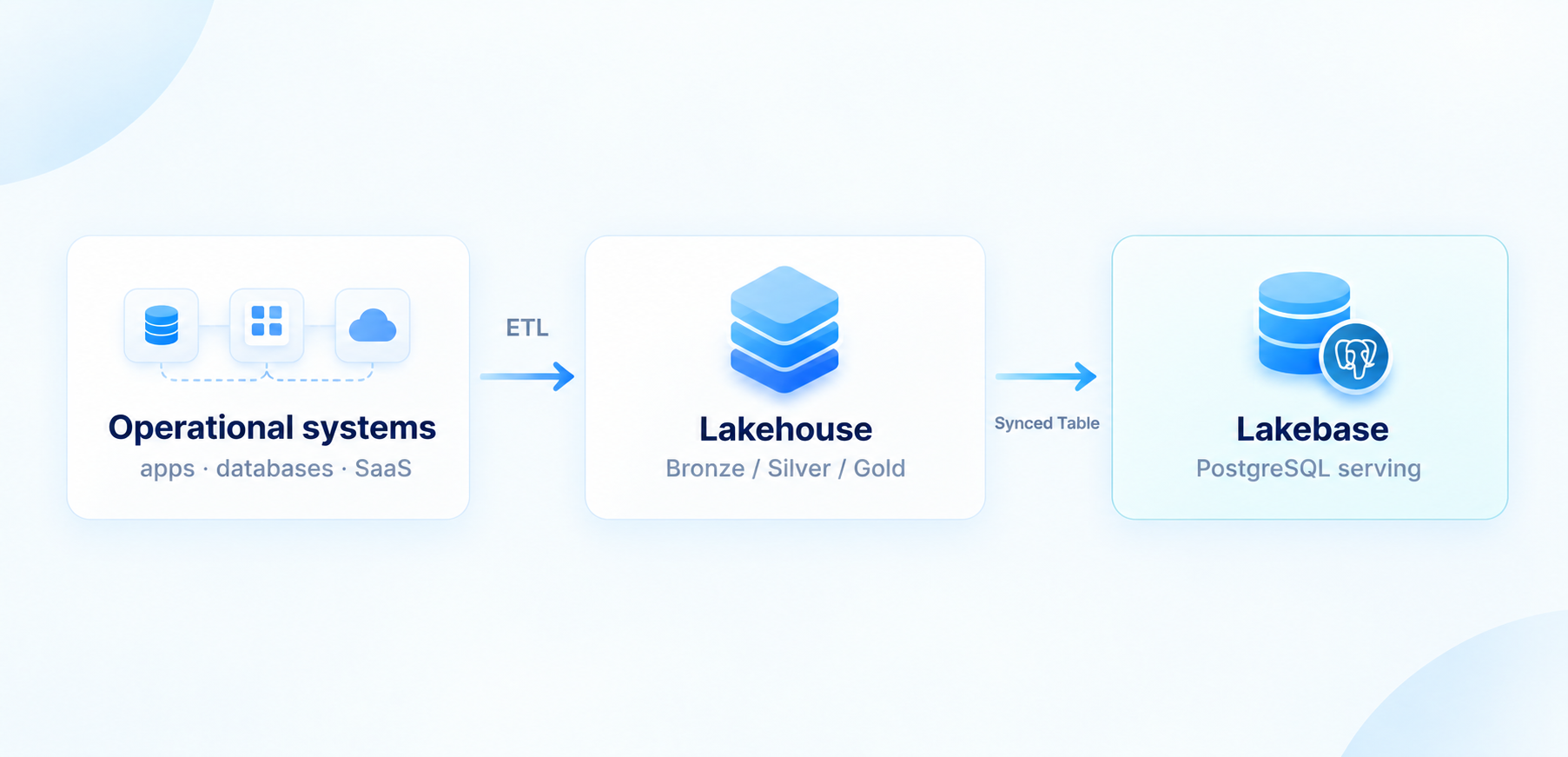
This is a reverse ETL pattern. Traditional ETL moves data from operational systems into the Lakehouse, and synced tables move selected analytical results back out in the serving direction. Databricks describes reverse ETL as syncing high-quality lakehouse data into the operational systems that power applications.
The pipeline you don’t have to write is the point. Most organizations already have a reverse-ETL job somewhere: a nightly notebook that writes to an RDS instance, built by someone who has since changed teams, monitored by nobody, and discovered to be four days stale on the morning a campaign depends on it. Synced tables replace that job with a managed object registered in Unity Catalog, so the serving copy sits under the same governance layer as the rest of your data.
Hands-on: serving a Customer 360 from Lakebase
The Gold table
Suppose the data engineering pipeline produces this Delta table:
| CREATE TABLE main.gold.customer_360 ( customer_id BIGINT, customer_name STRING, customer_segment STRING, lifetime_value DECIMAL(12,2), churn_probability DOUBLE, recommended_product STRING, updated_at TIMESTAMP ) TBLPROPERTIES (delta.enableChangeDataFeed = true);
INSERT INTO main.gold.customer_360 VALUES (1001, ‘Rahul Sharma’, ‘Premium’, 125000.00, 0.12, ‘Flagship handset’, current_timestamp()), (1002, ‘Priya Patel’, ‘Standard’, 45000.00, 0.42, ‘Wireless earbuds’, current_timestamp()), (1003, ‘Amit Shah’, ‘Premium’, 210000.00, 0.08, ‘Pro laptop’, current_timestamp()); |
The TBLPROPERTIES line matters. Triggered and Continuous sync modes need Change Data Feed enabled on the source table, and the synced-table dialog warns you if it is missing.
Creating the synced table
In Catalog Explorer, select main.gold.customer_360 → Create → Synced Table, and configure it. Databricks documents synced tables for AWS, Azure and GCP, so follow the synced tables documentation for your cloud.
| Setting | Value |
| Source table | main.gold.customer_360 |
| Primary key | customer_id |
| Lakebase project | customer-serving-project |
| Branch | Production |
| PostgreSQL database | customer_app |
| Destination table | main.gold.customer_360_synced |
| Sync mode | Snapshot, Triggered or Continuous |
Why the primary key matters
The primary key uniquely identifies individual records in the synchronization process. A good one is unique, stable and non-null: customer_id = 1001 should always mean the same customer. Rows with nulls in primary key columns are excluded from the sync.
If the source holds multiple records per key, configure a timeseries key as well so the latest version can be identified. In our table that would be updated_at, if it held several rows per customer. Without one, duplicate keys make the sync pipeline fail. With one, the synced table keeps only the row with the latest timeseries value for each key, at some cost in sync performance. As written, our table has one row per customer, so it needs none.
Choosing a sync mode: Snapshot, Triggered or Continuous
Pick the sync mode from the application’s freshness SLA and the source’s change pattern.
| Sync mode | Best for | Freshness | Change data feed |
| Snapshot | More than about 10% of rows change per cycle, or the source is a view | Full refresh each run | Not required, only SELECT |
| Triggered | Hourly updates or a refresh at the end of a pipeline | As fresh as the last run | Required |
| Continuous | Freshness requirement below the pipeline cadence | Seconds, 15-second minimum interval | Required |
Snapshot
Snapshot performs a full refresh of the source dataset. It fits when a large share of rows changes every cycle (Databricks suggests above roughly 10%, where it is up to 10 times more efficient) or when the source can’t provide a change data feed, as with views and materialized views. Snapshot only requires the source to support SELECT *.
Triggered
Triggered processes changes when the sync runs. It works well when the application tolerates periodic updates, such as hourly or on completion of a data pipeline. Databricks flags triggered syncs more frequent than every five minutes as costly, so consider Continuous at that cadence.
Continuous
Continuous suits applications that need fresher data than a scheduled run can give: recommendations, risk scores and live operational analytics. Latency is measured in seconds, with a minimum refresh interval of 15 seconds.
Triggered and Continuous both need a change data feed on the source. Enable Change Data Feed on eligible Delta tables, or use Automatic Change Data Feed on supported sources, which Databricks now recommends where available. Check its status in your workspace. Views and materialized views have no change data feed and can only sync in Snapshot mode.
Our default is Triggered, fired at the end of the pipeline that writes the Gold table. If a churn score is recalculated four times a day, Continuous mode pays to keep a sync pipeline warm so it can propagate four updates. Triggering the sync as the last pipeline step gives the application exactly the freshness the data has. Reach for Continuous when the freshness requirement sits below the pipeline cadence, and be ready to name the SLA when someone asks.
Querying from PostgreSQL
Once synchronized, the application queries an ordinary PostgreSQL table:
| SELECT customer_id, customer_name, customer_segment, churn_probability, recommended_product FROM gold.customer_360_synced WHERE customer_id = 1001;
/* returns: 1001 | Rahul Sharma | Premium | 0.12 | Flagship handset */ |
The synced table lands in a Postgres schema named after its Unity Catalog schema, so main.gold.customer_360_synced is queried as gold.customer_360_synced.
Connecting from an application
The client side is a standard PostgreSQL connection:
| import psycopg
conn = psycopg.connect( host=LAKEBASE_HOST, # your compute endpoint dbname=”customer_app”, user=SERVICE_PRINCIPAL, password=oauth_token(), # short-lived OAuth token sslmode=”require”, )
with conn.cursor() as cur: cur.execute( “SELECT customer_name, customer_segment, churn_probability ” “FROM gold.customer_360_synced WHERE customer_id = %s”, (1001,), ) print(cur.fetchone()) |
Design for credential expiry on day one. Lakebase authenticates with OAuth tokens that expire after one hour. Expiry is checked at login, so open connections stay alive, but a long-running application needs a fresh token each time its connection pool opens a new connection. It’s small work and an annoying thing to discover in production.
Native Postgres password roles exist for clients that can’t refresh credentials hourly, and they also work with PgBouncer pooling, which OAuth tokens don’t. New projects have password roles disabled by default.
When the Gold data changes
Suppose the ML pipeline recalculates a customer’s churn probability:
| UPDATE main.gold.customer_360 SET churn_probability = 0.78, recommended_product = ‘Premium retention offer’, updated_at = current_timestamp() WHERE customer_id = 1001; |
With Triggered or Continuous mode, the update propagates into Lakebase and the application picks up the new result through PostgreSQL, without knowing how the number was calculated. Your data science team can change the model, the features, even the library, and the application contract stays one row and five columns.
Mixing synced data with application tables
Lakebase also holds application-owned PostgreSQL tables next to synced data:
| CREATE TABLE public.customer_session ( session_id UUID PRIMARY KEY, customer_id BIGINT, device_type TEXT, login_time TIMESTAMP ); |
That table is application-owned and supports normal INSERT, UPDATE, DELETE and SELECT. Meanwhile gold.customer_360_synced carries analytical information from Databricks, and the application joins the two:
| SELECT s.session_id, s.device_type, c.customer_name, c.customer_segment, c.churn_probability, c.recommended_product FROM public.customer_session s JOIN gold.customer_360_synced c ON s.customer_id = c.customer_id; |
Application state plus Lakehouse intelligence, joined in a single PostgreSQL query. Most teams end up building this pattern.
| Treat synced tables as read-only Modifying a synced table directly in Postgres is possible, but Databricks strongly recommends running only read queries, so use them as serving tables. Anything transactional belongs in an application-owned table. Design the boundary deliberately, because teams that skip this step find it halfway through a sprint. |
Lakebase vs running PostgreSQL yourself: when does it pay off?
Sometimes running your own PostgreSQL is the right call. Lakebase earns its place when:
- The data your application serves is produced by the Lakehouse, and its freshness is a product requirement.
- You would otherwise own the export pipeline yourself, with backfills, failure alerting and the rest.
- Governance Synced tables are registered in Unity Catalog, so the serving copy stays visible to your governance tooling. Access on the Lakebase side runs through Postgres roles, so plan permissions on both sides.
- Non-production environments carry real cost or friction. Branching plus scale-to-zero is a different economic model from running four always-on instances.
It earns less when your application’s data is overwhelmingly transactional and touches analytics rarely, when you already operate a mature PostgreSQL platform with the people and tooling around it, or when you depend on extensions and version control that a managed service won’t hand you. Lakebase is a serving layer with a database attached. Position it beside your core OLTP estate, because pitching it internally as a full replacement is the fastest way to lose the argument.
Lakebase synced tables: limits and gotchas to plan for
- The sync pipeline is a separate cost. It doesn’t appear in your database compute figure, and Continuous mode raises spend to lower latency. Budget it explicitly and watch it with data observability like any other production pipeline.
- Continuous has seconds of lag. Updates arrive within seconds, so an application that must read its own write should store that write in an application-owned table.
- Change Data Feed is a prerequisite. Triggered and Continuous modes need it on the source table, and views and materialized views sync in Snapshot mode only.
- Region and feature availability move quickly. Lakebase shipped high availability, compliance profiles and SOC 2 Type 2 coverage during 2026, according to the release notes. Check what your region and tier offer before designing around it.
- Connection limits scale with compute size. A database sized for data volume can still be sized wrong for concurrency. With autoscaling, the limit follows the smaller of your maximum CU and eight times your minimum CU, and each synced table can use up to 16 connections.
- Schema changes are additive only. In Triggered and Continuous modes, adding a column flows through. Changing a key or making any other non-additive change means deleting and recreating the synced table.
- Sync throughput is finite. Incremental syncs write roughly 150 rows per second per CU, and Snapshot syncs reach up to 2,000 rows per second, so size for the initial backfill and for high-churn tables as well as steady-state reads. A single source table can have up to 20 synced tables, and Databricks recommends keeping tables that need refreshes under 1 TB, per the synced tables limits.
Where Lakebase fits: use cases for serving lakehouse data
Lakebase becomes useful wherever data engineering, ML or AI output needs to reach an operational application.
Customer 360 for CRM and web apps
The Lakehouse calculates the customer profile, and Lakebase serves it to the CRM or web application.
Real-time recommendations
Recommendations generated in Databricks reach an e-commerce application through PostgreSQL, with no bespoke serving infrastructure in between. The scoring side is where predictive analytics work lives.
Risk and fraud scoring
Applications retrieve the latest calculated risk score without querying analytical infrastructure inside a request path.
AI applications and agents
Lakebase can hold analytical context and agent state together, a combination that is awkward to assemble anywhere else. An agent that needs a customer’s segment and churn score next to its own conversation state gets both from one connection. Teams building these systems can start with AI application development patterns.
Healthcare data serving
Curated patient data, encounters, risk scores and care recommendations can be computed in the Lakehouse and served to authorized applications. Lakebase supports workspaces with the compliance security profile set to HIPAA, C5 or TISAX, and it is SOC 2 Type 2 compliant.
Platform compliance covers the platform. Your application still needs its full PHI review against the safeguards in the HIPAA Security Rule. Our guide to PII and PHI protection in healthcare is a good place to start the full PHI review for the healthcare domain.
What Databricks Lakebase costs: compute, storage and the sync pipeline
Lakebase pricing is consumption-based, built primarily on compute and storage. Databricks bills pay as you go with a 14-day free trial, and the pricing page carries current rates by cloud and region.
Cost ≈ compute + storage + snapshots + optional HA and read replicas + the sync pipeline
Compute units and Lakebase autoscaling
Compute is measured in Compute Units (CU). Each CU allocates roughly 2 GB of RAM along with associated CPU and local SSD.
| Compute | Approx. RAM |
| 0.5 CU | ~1 GB |
| 1 CU | ~2 GB |
| 2 CU | ~4 GB |
| 4 CU | ~8 GB |
| 8 CU | ~16 GB |
| 16 CU | ~32 GB |
| 32 CU | ~64 GB |
Commonly used sizes. The Lakebase App shows a subset. Through the API, Terraform, Asset Bundles or the SDK you can set any integer CU value: 1 to 64 for autoscaling, 65 to 112 for larger fixed-size computes.
Sizes start at 0.5 CU and rise in integer increments. Autoscaling reaches 64 CU (128 GB), and larger fixed-size computes go up to 112 CU. Confirm sizing in the Databricks compute documentation before you set a budget.
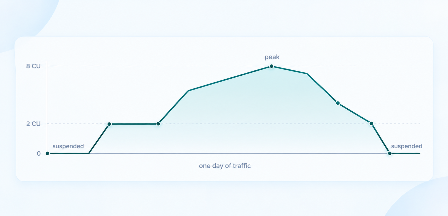
Configure a production database between, say, a 2 CU minimum and an 8 CU maximum (the gap between minimum and maximum cannot exceed 16 CU). Lakebase watches CPU load, memory use and working set size to decide when to scale. During quiet periods the database sits near the floor, and as traffic rises Lakebase adds capacity and later gives it back. Conceptually:
compute cost ≈ actual CU consumption × active time × CU rate
The database doesn’t need to stay sized for peak demand all day.
Scale-to-zero
Lakebase can suspend compute when a workload is idle, which suits development, testing, proofs of concept, internal tools and anything intermittent. A development database used only during working hours suspends after its configured inactivity period. New instances default to a 24-hour idle timeout, which you can set anywhere from 60 seconds to 7 days. While suspended, compute charges stop, though durable storage remains billable.
Scale-to-zero is available only when a compute’s maximum size is 32 CU or smaller, and a suspended database restarts at its minimum autoscaling size on the next connection. That wake-up is why production databases usually leave it off. High availability configurations don’t support scale-to-zero at all.
For non-production estates, this is often where the business case lives, well before anyone measures a latency gain in production.
Always-On pricing for production
Scale-to-zero suits new or intermittent workloads. An established production database with a steady floor of traffic never idles, so scale-to-zero saves it nothing. Turn scale-to-zero off and set the autoscaling range. After 24 hours of continuous use, the baseline (your minimum CU) bills at a rate 25% lower than standard Autoscaling, and anything above the baseline bills at the standard rate. HA replicas and the largest instances qualify automatically. Databricks is also running a 50% promotional discount through 31 January 2027 that stacks on top. Set the minimum from a baseline you have observed, because you pay for it whenever the compute runs.
The costs teams forget
- Synced table pipeline: its own compute, outside your database figure.
- Storage: PostgreSQL data stays in durable storage even while compute is suspended.
- Snapshots: snapshot and backup retention adds to storage consumption. Databricks’ cost optimization guide puts snapshot storage at 74% less than branch storage, so match recovery windows to real incident needs.
- High availability: production HA adds one to three secondary computes, and HA computes don’t scale to zero.
- Read replicas: read-heavy applications add replica compute.
- Branches: storage-efficient thanks to copy-on-write, but active branch compute still costs.
As a Databricks partner, we recommend one saving worth taking early: sync only the working set the application needs. A rolling window, for example 60 days, keeps Lakebase storage small while the full history stays in the Lakehouse.